ステレオネットの構造をよく理解するためには，自作してみるのが良いかもしれない。 手描きで自作することも不可能ではないだろうが，より簡単にパソコンなどを利用してステレオネットを描いてみよう。 ここでは，実習でも使用するウルフの赤道投影ネットを描くことを考える。

これまでに 2.1. で見てきたように，赤道投影ネットには， 投影面と平行な直線 \(\mathrm{M}\) を含む平面と球面との交円 (大円群) と， \(\mathrm{M}\) を法線とするような平面と球面との交円 (小円群) が描かれている ( 図 2.1.3. )。 このうち大円群は等角投影用のウルフのステレオネットであれば，直線 \(\mathrm{M}\) を \(y\) 軸として，\(xy\) 平面を投影面とすれば， 式 (1.3.19) を参考に投影面と投影する面との交角を \(\theta\) として，

\begin{align} (x - (-r \tan \theta))^2 + y^2 = r^2 (1 + \tan^2 \theta) \tag{2.2.1} \end{align}

という式を利用して描くことができることがわかる。基円の半径 \(r = 1\) とすれば，

\begin{align} (x + \tan \theta)^2 + y^2 = 1 + \tan^2 \theta \tag{2.2.2} \end{align}

である。

また小円群は 式 (1.3.15) の \(\alpha = 0\) で \(R = r = 1\) のときを考えればよいから，

\begin{align} x^2 + \left( y - \frac{\cos 0}{\sin 0 + \cos \gamma} \right)^2 & = \frac{\sin^2 \gamma}{(\sin 0 + \cos \gamma)^2} \\ \nonumber x^2 + \left( y - \frac{1}{\cos \gamma} \right)^2 & = \tan^2 \gamma \tag{2.2.3} \end{align}

を使って描くことができる。

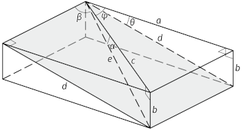
大円群も小円群も基円の外側には出ないことを考えれば， 大円群の大円はそれぞれ \(-1 \le y \le 1\) の範囲で描けば良く， 小円群の小円は \(y \gt 0\) では \(y \le \cos \gamma\)， \(y \lt 0\) では \(y \ge \cos \gamma\) の範囲のみ描けば良い。 大円群はゼロ点付近で線が密になって見づらいので， 省略することもできる。 例えば，直線 \(\mathrm{M}\) と交角\(\beta\) で斜交する線の回転の軌跡である小円までで止めるなら， 面 ( 1.3.1. でいうところの面 \(\mathrm{P}\)) 上にあるそのような線 (やはり 1.3.1. でいうところの線 \(\mathrm{L}\)) の トレンド \(t\) とプランジ \(\alpha\) がわかれば \(y\) 座標が決まる。そこで 図 1.3.6. と同様に考えると ( 図 2.2.1.)，

\begin{align} \sin \alpha = \frac{b}{e} & = \frac{b}{d} \times \frac{d}{e} \\ \nonumber & = \sin \theta \sin \beta \tag{2.2.4} \end{align}

である。したがって，\(\alpha = \sin^{-1} (\sin \theta \sin \beta)\) である。

\(\alpha\) がわかれば， 式 (1.3.4) から \(t = \sin^{-1}(\tan \alpha / \tan \theta)\) である。 直線 \(\mathrm{L}\) の投影点と基円の中心との距離は \(r = 1\) のとき 式 (1.3.1) より \(\cos \alpha / (1 + \sin \alpha)\) なので， そのときの \(y\) 座標を \(y_\mathrm{lim} = \cos \alpha \cos t / (1 + \sin \alpha)\) とすれば， 大円は\(-y_\mathrm{lim} \le y \le y_\mathrm{lim}\) の範囲で描けば良いことになる。

以上の考え方を利用して，例えば Julia を使えば次のようにウルフの赤道投影ネットを描くことができる ( 図 2.2.2.)。 ここでは大円群も小円群も \(5^\circ\) 刻みとし， 大円群は \(n \times 10^\circ\) のものを \(5^\circ\) の小円まで， それ以外を \(10^\circ\) の小円まで描いている。 また，基円および大円群と小円群の鉛直面の大円は，それぞれ別に描いている。 なお，これを試すには Julia や必要なパッケージ (Plots と ImplicitPlots) のインストールが必要だが， それらについては親切なウェブサイトがいくらでもあるので， そちらを参考にされたい。

            # Wulff equatorial net with 5-degree intervals
            
            # Load packages
            
            using Plots, ImplicitPlots
            
            # Define functions
            function prim_circ(x, y)
                # Equation for the primitive circle
                return x^2 + y^2 - 1
            end
            
            function x_axis(x, y)
                # Equation for the x-axis (vertical plane)
                return y
            end
            
            function y_axis(x, y)
                # Equation for the y-axis (vertical plane)
                return x
            end
            
            function great_circ(x, y, θ)
                # Equation for a great circle
                #   based on a given angle of intersection θ
                # See equation (2.2.2)
                return (x + tan(θ))^2 + y^2 - (1 + tan(θ)^2)
            end
            
            function small_circ(x, y, γ)
                # Equation for a small circle
                #   based on a given angle of intersection γ
                # See equation (2.2.3)
                return x^2 + (y - (1/cos(γ)))^2 - tan(γ)^2
            end
            
            # Initial plot with the primitive circle and axes
            plt = implicit_plot(prim_circ;
                                 xlims = (-1, 1), ylims = (-1, 1), linewidth=1)
            implicit_plot!(plt, x_axis; xlims = (-1, 1), linewidth=1)
            implicit_plot!(plt, y_axis; ylims = (-1, 1), linewidth=1)
            
            # Plot great circles
            for i in 1:17
               θ = i * (π / 36)  # 5-degree intervals
                 
                # Define functions for right and left part of the Wulff net
                gc_right(x, y) = great_circ(x, y, θ)
                gc_left(x, y) = great_circ(x, y, -θ)
              
                # Adjust line thickness for alternating intervals
                if mod(i, 2) == 0
                    β = π / 36
                    line_thickness = 0.75
                else
                    β = π / 18
                    line_thickness = 0.5
                end

                # Calculate y-axis limit
                # See equations (2.2.2), (1.3.4), (1.3.1)
                α = asin(sin(θ) * sin(β))
                t = asin(tan(α) / tan(θ))
                y_lim = cos(α)/(1 + sin(α)) * cos(t)

                # Plot great circles in respective parts of the net
                implicit_plot!(plt, gc_right;
                                xlims = (0, 1), ylims = (-y_lim, y_lim), 
                                linewidth = line_thickness)
                implicit_plot!(plt, gc_left;
                                xlims = (-1, 0), ylims = (-y_lim, y_lim), 
                                linewidth = line_thickness)
            end
            
            # Plot small circles
            for i in 1:17
                γ = i * (π / 36)  # 5-degree intervals
                
                # Define functions for upper and lower parts of the Wulff net
                sc_upper(x, y) = small_circ(x, y, γ)
                sc_lower(x, y) = small_circ(x, -y, γ)
                
                # Adjust line thickness for alternating intervals
                if mod(i, 2) == 0
                    line_thickness = 0.75
                else
                    line_thickness = 0.5
                end
                
                # Calculate y-axis limit
                y_lim = cos(γ)
                
                # Plot small circles in respective parts of the net
                implicit_plot!(plt, sc_upper;
                                xlims = (-1, 1), ylims = (0, y_lim), 
                                linewidth = line_thickness)
                implicit_plot!(plt, sc_lower;
                                xlims = (-1, 1), ylims = (-y_lim, 0), 
                                linewidth = line_thickness)
            end
            
            # Final plot
            plot(plt, aspect_ratio=:equal, framestyle=:none, legend = false, 
                  xlims = (-1.1, 1.1), ylims = (-1.1, 1.1), size = (300, 300), 
                  grid = false, ticks = nothing)
          

パソコンなどを利用したステレオネットの描画には，これ以外にも様々な方法が考えられる。 また，大円群・小円群を \(1^\circ\) 刻みにしてみる，極投影ネットを描いてみる， シュミット・ネットを描いてみる，などいろいろと試してみると， ステレオネットや球面投影について理解しやすくなるかもしれない。